Identifying sales trends can be complicated, particularly if your company’s sales totals vary drastically from week to week, month to month, etc. Have you ever wanted to look at sales figures in a report, and also get an average per week/month/quarter of those figures? I once had that issue with a particular product line – one month might seem slow, but without doing a lot of manual calculation, there was no way of knowing how far from the average that month really was. And then… I attended an awesome reporting session at Dreamforce – feel free to watch the recording before you try this at home – and finally learned how the PREVGROUPVAL function works! Here’s how to add moving average information to a report, with a nifty combination chart as well.

1. Start with a report that is summarized by date – mine was summarized by calendar month. With details hidden, it looked like this:

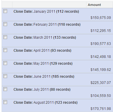
Well that’s just fine – but what if I wanted to see what the average per month was – say, every three months? I’d have to get a calculator and figure that out for each 3-month period in my report. No thank you!

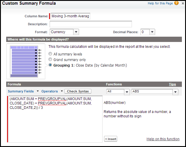
2. Customize your report, and under Fields over on the left, double click on Add Formula. Give your formula a name – mine was “Moving 3-month Average.” Select the format “Currency” and specify how many decimal places to display. In the options for where to display your formula, select “Grouping 1: Close Date.”

Then you will want to write your formula. The formula section has tools that will insert fields and functions for you. Follow these steps:

• Start with “ ( “
• From the Summary Fields list, select Amount > Sum
• Enter “ + “
• From the Functions list, select PREVGROUPVAL, and click < Insert
• In the function that you have just inserted, highlight the text that says summary_field – then from the Summary Fields list, select Amount > Sum to replace the highlighted text
• At the end of the formula, enter “ + “
• From the Functions list, select PREVGROUPVAL, and click < Insert
• In the function that you have just inserted, highlight the text that says summary_field – then from the Summary Fields list, select Amount > Sum to replace the highlighted text
• In the function that you have just inserted, click after “CLOSE_DATE” and enter “,2”
• At the end of the formula, enter “ ) / 3 ”

Check the screenshot below to make sure your formula matches… then click OK.

If you run your report now, it will look like this:

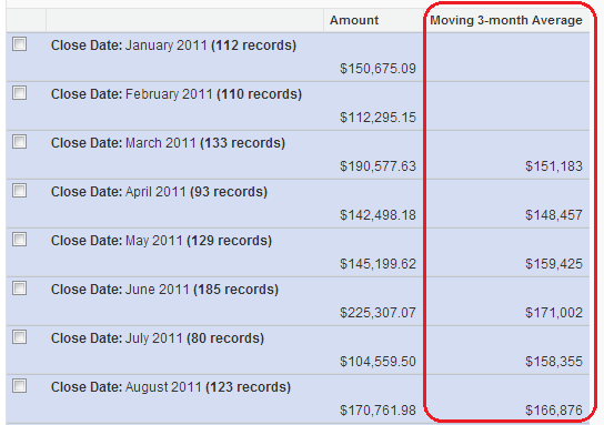
The reason the first two rows do not have a Moving 3-month Average is, they do not have two previous rows to average their amounts with (the formula takes the current month, adds the two previous months, and returns an average of the three of them).

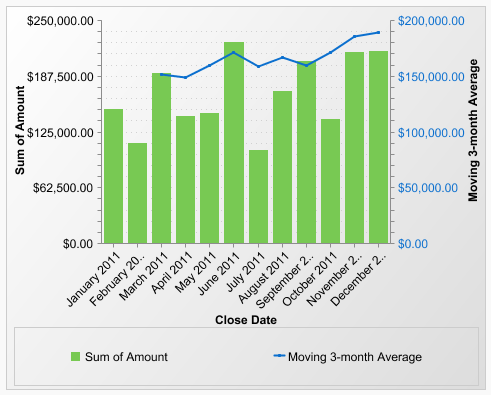
3. Now if you’d like to add a chart, go back into Customize and click Add Chart (or Edit Chart) if you already have one. This works best with a vertical bar chart. On the Chart Data tab, check the “Combination Charts” box and fill in the information as pictured below, then click OK. (Hint: you may also want to go to the Formatting tab and change the Legend Position to Bottom.)

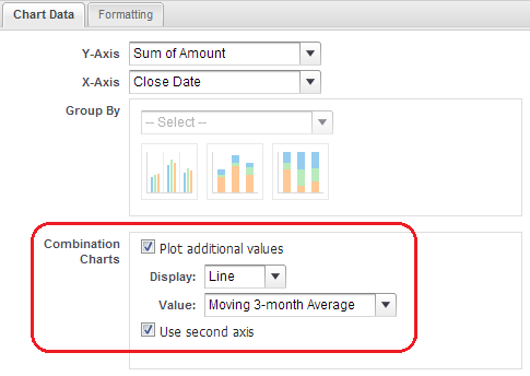
Voila! Your chart will look something like this:

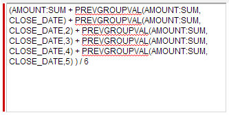
One more tip: Let’s say you wanted more than 3 time periods in your formula. You can just keep repeating the process until you have as many AMOUNT: SUM calculations as you like. For instance, if I wanted a moving 6-month average, my formula would look like this: